Notes to myself, as I try to understand quantum computing without succumbing to mystification.
1 Introduction
In as few words as possible, I hope to answer some practical questions I had when I started reading up on the topic. Like these:
How are quantum computers built?
Are we going to have quantum laptops any time soon?
How can I get my hands dirty with quantum computing today? What do I need to understand to write my first “Hello world” quantum computing program?
What advantages, if any, does quantum computing offer? This topic is key to the whole thing, but I’m going to skip over it very lightly here. Maybe a Part II will discuss it in more depth.
What is the status and what are the prospects of quantum computing today? Well, an answer is too much to hope for, but I’ll offer some reflections.
But let’s start with three building blocks of quantum computers: qubits, gates, and circuits.
2 Building blocks
2.1 Qubits
Regular computers are built around bits, quantum computers are built around qubits. So what does that mean?
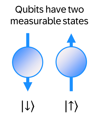
The archetypal example of a qubit is an atomic nucleus with a spin of ½, like the 89Y isotope of Yttrium (although many quantum computers don’t actually use spin-½ nuclei, but let’s put that aside for now). The spin means that the nucleus has angular momentum, as if it were an electrical charge spinning in one direction or the other. This spinning electrical charge creates a little magnet that can be pointing either “up” or “down”.
(Aside: classically, the axis around which the rotation happens is the “direction” of angular momentum, which is a bit odd when you first come across it. Angular momentum in quantum mechanics follows the same rule. Similarly, a classical electric current moving in a circle creates a magnetic field. So quantum spin, a form of angular momentum, is following similar rules as classical angular momentum. A big difference, though, is that classical angular momentum can take any value–a bicycle wheel can spin at any speed–but quantum spin can take only specific discrete values (it is “quantized”): in the case of a spin-½ particle that is +½ or -½, which we usually call “spin up” or “spin down”. These two values can represent \(0\) and \(1\) when used as a qubit in a quantum computer, just as a classical “bit” might be a transistor that can take on a state of “on” or “off”. It’s often said that an electron or nucleus with angular momentum is like a little ball spinning around an axis, except that it’s not a ball and it’s not spinning.)
Qubits, as has often been said, exist in a state that is a superposition of 0 and 1, but let’s leave that to one side for now as well.
Qubits may be atomic nuclear spins, using nuclear magnetic resonance, but in principle any other system that displays this two-level behaviour can be used as a qubit. Some research groups have built quantum computers with atomic-scale qubits, like arrays of charged ions trapped in space by electromagnetic fields (e.g., Quantinuum or IonQ) or arrays of neutral atoms (e.g. QuEra). Others (e.g. Google and IBM) are exploiting macroscopic quantum phenomena – for example, qubits based on superconductivity in circuits of maybe a micrometre in size: the current in a superconductor is macroscopic (although still small by our standards) but is quantized. And there are other approaches too : photonics (e.g. Photonic and Xanadu), topological “anyons” (Microsoft) and more. These different approaches are often called “modalities” in industry jargon.
A feature of quantum computing is its division of intellectual and physical labour. Some people build quantum computers using a particular modality, and learn how to work with the components that they need. Others spend their time developing quantum algorithms that could, in principle, run on a quantum computer built with any of these modalities.
The large number of qubit “modalities” being pursued is often seen as a strength of the field, a sign of its vitality, and this makes sense from a “don’t put all your eggs in one basket” perspective. The number of modalities increases the chance that one of them will surely a scalable quantum computer. But I wonder… is it also a sign of the uncertainty that remains? After all, if there were a clear path from a particular modality to a general purpose quantum computer, then the industry would have coalesced around that modality. The number of modalities being actively pursued suggests that each has obstacles that it has not yet surmounted. It would be interesting to chart the progress in the industry, not by what each company and research group says about its own modality and its own breakthroughs, but by what they each say about the limitations of everyone else who is competing for the same funds. But OK, back to quantum computing proper.
2.2 Gates
Whatever approach you choose, you want to build a computer out of these qubits. So the next thing you need for a computer is logic gates. In a classical computer the simplest gate is this NOT gate.
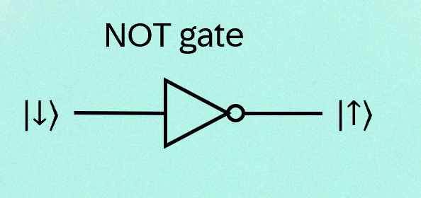
The NOT gate has one input and one output. If the input is 0, then the output is 1, and if the input is 1 then the output is 0.
In classical computers, the lines are wires and the shield-symbol is etched into a chip and the bits are charges moving through the gates. In the world of quantum computers, the qubits stay where they are: it’s called “in-place computing”. If you shine a laser at one particular qubit and cause it to flip from one of its states to the other, then that’s like a NOT gate: it turns a 0 into 1 or a 1 into 0. In quantum computing circuit diagrams, the lines are not wires, they are before and after states of the qubit.
(In the figure above, the state of each qubit is represented in what’s called the “Dirac ket notation”, like \(| \uparrow \rangle\) or, equivalently, \(| 1 \rangle\). This notation is really useful and standard in all areas of quantum mechanics, but here it’s just a symbol that shows the value of a qubit.)
Most classical gates, like XOR and NAND, have two inputs, and many quantum gates can also have two inputs. Here is a “Controlled NOT gate” or CNOT gate, which is an important component of quantum computers. If the top qubit is spin down (0), the bottom qubit is unchanged. If the top qubit is spin up (1), the bottom qubit is flipped.
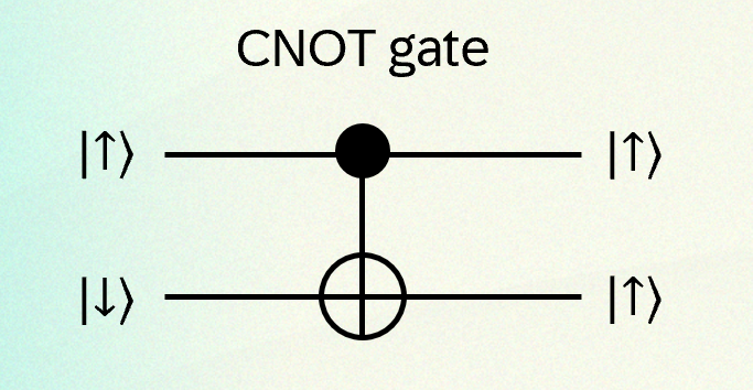
Again, if this were a classical computing gate, the “bits” would be charges travelling along wires, going in to the gate from the left and out on the right. But in quantum computing the gate is not a feature of a circuit etched into a chip. It’s an operation—a combination of laser or microwave pulses that changes the state of the qubits from a before state (on the left) to an after state (on the right)—and the qubits stay in place.1
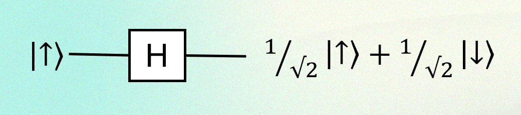
Before moving on, I should mention one gate you will see all the time in quantum computing, but not in classical computing. It’s called the Hadamard gate. If you prepare an input qubit in state \(| \uparrow \rangle\) then a Hadamard gate puts it into a superposition of states. Many circuits start with Hadamard gates way to take advantage of this superposition. I just mention this because it is useful and ubiquitous, and also because it is needed in the next section.
2.3 Circuits
Once you have qubits and gates, the next thing to do is implement algorithms. In classical computers you have a fixed circuit and programming instructions send bits through these fixed gates to implement an algorithm. In a quantum computer, you start with a set of qubits in a prepared state (usually all \(|0\rangle\)), and apply a sequence of gate operations and then measure the output. So a circuit is how you implement an algorithm.
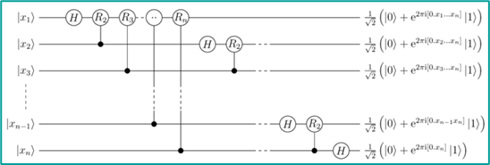
Here is a circuit diagram for a quantum fourier transform (QFT), which turns out to be important in the Shor algorithm for factoring integers. You have \(n\) qubits, you prepare them in some initial state \(| x_i \rangle\), you subject them to a series of gates, and you end up with some outputs which you measure.
To be useful, a quantum computer would need many qubits and many gates, and so far there are strict limits on how many qubits can be assembled, and how many gates can operate on them before they lose their well-defined state. How many and why? We’ll come to that later on.
3 Will I have a quantum laptop? (No)
When I started looking at quantum circuit diagrams I thought it contradicted the idea of quantum computers as general purpose computers, because you need different circuits for different algorithms and I assumed that any computer would have a fixed set of circuits (like CPU circuits are etched into silicon) and hence be limited in what algorithms it can execute.
But once I realised that a circuit is not a permanent thing but is instead a sequence of operations (gates) that implement an algorithm, then I realised it’s not a contradiction at all.
Perhaps I’m belabouring this point, but for some reason, many introductions to quantum computing seem to skip over this difference between regular electrical circuits, and “quantum circuits”. I read several before I realized what was going on.
So are quantum computers general purpose? Well yes and no. Formally, they are. That is, there is a set of gates (different to the gates for classical computing) which satisfy the requirements for Turing completeness. So that’s nice.
But what about “general purpose” in the more everyday, practical sense? Let’s go back to how you build quantum computers. No matter what approach you take, the set of qubits must exist in what is called a single “quantum state”, and quantum states fall apart or “decohere” if they interact with the wider world, so they have to be isolated. Also, thermal energy (which is just one form of interaction with the wider world, of course) will jiggle these qubits among the states and you can’t have that, so quantum computers have to be operated at very low temperatures, meaning about 1K.2
This fragility of quantum states has consequences:
You won’t, in the foreseeable future, have a quantum computing laptop. Quantum computers need cooling and will be built in fixed locations.
It’s going to be expensive to build them. And so your company probably won’t be buying many quantum computers any time soon. It makes sense to have specialised providers who will provide time on them through a cloud service.
For any algorithm that can be executed either classically or in a quantum computer, classical is going to be roughly a gazillion times cheaper for the foreseeable future. You won’t be running most of your code on a quantum computer.
BUT there are certain tasks that may be done more quickly on a quantum computer than on a classical one, if a powerful enough quantum computer can be built. So what will most likely happen is that specific function calls within a larger program may be executed on a quantum computer, and the rest will be done on a classical one.
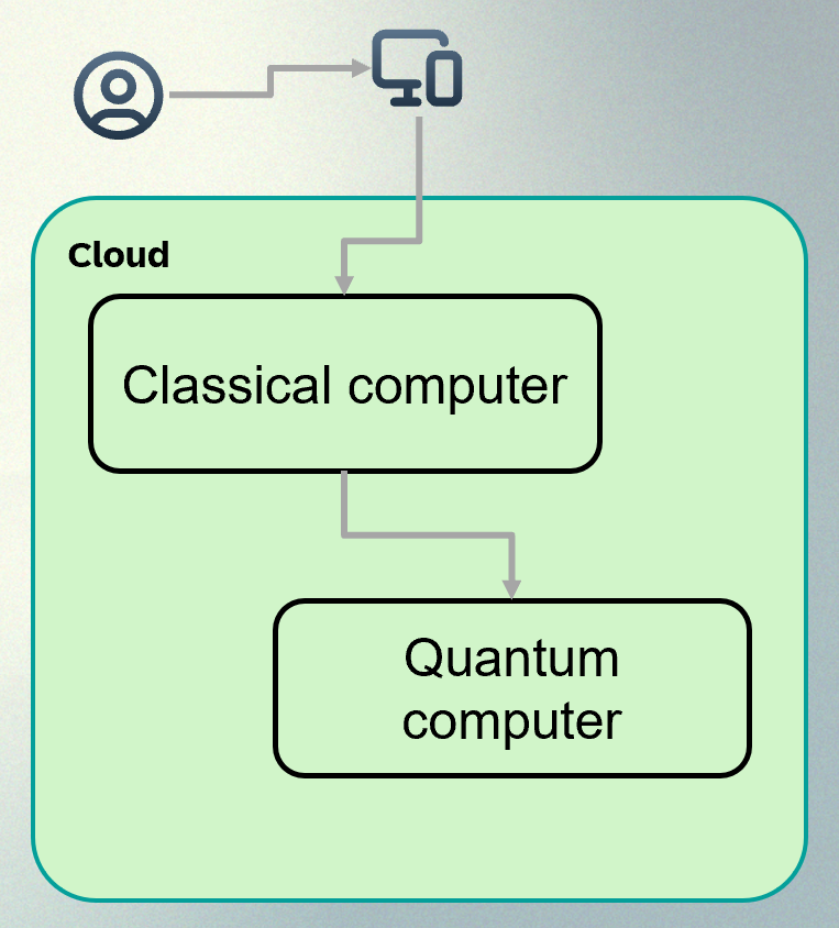
The emerging paradigm, at least as at October 2024, is of a cloud-hosted data centre where an application can use classical computers for many parts of an application, but have access to quantum computers to run specific functions. Perhaps it’s not surprising that Microsoft, IBM, and Google are at the forefront and Amazon (AWS) is now investing heavily: they want to host them, and rent them out to their cloud users.
4 How do I program a quantum computer?
The companies providing quantum computers want people to use them, so they provide libraries or modules that you can use. For example, Google and IBM provide python libraries (cirq and Qiskit, respectively) and Microsoft provides its own Quantum Development Kit. These libraries provide an interface to the host quantum computers and, more practically for most of us, provide a way to simulate quantum computing on a local classical computer, for small cases.
So here is some code that uses Google’s cirq library for python. It defines two qubits and a list of gates that operate on those qubits. Then it creates a circuit from the gates, and runs the circuit on a simulator on your local computer. As the algorithm is very simple, the quantum computation can easily be simulated on a classical computer. If you’re familiar with the python programming language, you can easily install cirq by typing pip install cirq at a command prompt. Here is a “hello world” example to give you an idea of what the code looks like, which each step described by a comment.
Providing quantum computing at the level of a library makes it possible to implement hybrid applications (which, as the last section showed, are the most likely form) with the quantum components implemented as functions of a largely-classical application.
import cirq

# Define two qubits
q_control = cirq.NamedQubit('control')
q_target = cirq.NamedQubit('target')

# Define a list of gates: a "Hadamard" gate on each qubit,
# followed by a CNOT gate, and then a measurement of the
# control qubit q_control.
gates = [
        cirq.H(q_control),
        cirq.H(q_target),
        cirq.CNOT(q_control, q_target),
        cirq.measure(q_control)
        ]

# Create a circuit from this list of gates
circuit = cirq.Circuit(gates)
print(circuit)

# Simulate the execution of the circuit
simulator = cirq.Simulator()
result = simulator.run(circuit)
print(result)
The “print” instructions display an ascii-art rendering of the circuit and the results. I found this exercise helpful, to see how an end user might construct a circuit in software and run it (albeit on a simulator). It does prompt the question: if all the quantum algorithms are going to be expressed in this unfamiliar circuit form, how expressive is this language? There is a big gap between “it’s a formally complete set of gates so you can do anything this way” and any more practical statement about real implementations.
5 Why might quantum computing matter?
Building a new kind of computer, defining new ways to express algorithms, providing new coding libraries, integrating computers with existing cloud services… this is all a lot of work. Why would you bother? Only because quantum computing has been shown to have an intrinsic advantage over classical computing, in principle, for certain kinds of problem. If I write up Part II of this introduction (link to come) then it will describe this advantage in detail, but here we shall skip lightly over the essential details. They are available in many other places anyway. The goal here is to get down the basic minimum that I needed to understand some of the descriptions you see elsewhere.
5.1 Superposition and interference
The idea of quantum advantage relies on a combination of two phenomena that are consequences of the wave/particle nature of quantum systems.
One is that qubits exist in superpositions of states. That is, although any measurement of the qubit will show it to be in state \(| \uparrow \rangle\) or \(| \downarrow \rangle\), in general the qubit can be in a state that is a superposition of these two, and it has what is called a wavefunction or (equivalently) a state vector \(| \psi \rangle\) (the Greek letter psi) given by:
\[ | \psi \rangle = \alpha | \uparrow \rangle + \beta | \downarrow \rangle \]
The \(| \uparrow \rangle\) and \(| \downarrow \rangle\) states, which are the only possible outcomes of measurement, are called eigenstates or, sometimes, basis states 3. The coefficients \(\alpha\) and \(\beta\) are probability amplitudes, meaning that in any measurement of the state of \(| \psi \rangle\) the probability of seeing state \(|\uparrow \rangle\) is \(\alpha^2\) and the probability of seeing state \(| \downarrow \rangle\) is \(\beta^2\). Sometimes these are also called phases. This is something you just have to take on trust unless you want to dive properly into quantum mechanics.
Some influential descriptions say that quantum computers carry out many calculations in parallel, and this notion of superposition is where the idea of quantum parallelism comes from: that you can act on \(| \uparrow \rangle\) and \(| \downarrow \rangle\) at the same time because the qubit is in a superposition of states. You may even have heard some people talk about “many worlds” interpretations of quantum mechanics in which qubits are simultaneously “computing” each possible value of \(\alpha\) and \(\beta\) in different universes.
I really think it is best to put these aside as unnecessary (and unjustified) science-fiction-inspired enthusiasms. Practically, from what I can see, superposition alone does not deliver massive parallelism. First, the qubit is not “in both states at once”, it is in one state with one probability, and the other state with a different probability, and in any measurement you only ever see either one of the two eigenstates \(| 0 \rangle\) or \(| 1 \rangle\): you can only ever get one bit of information out of qubit. (This is far from an original observation.)
The second quantum phenomenon is interference, and here things get more messy. First, there is the notion of a quantum “state”: a system is only “in a (pure) quantum state” if it is isolated from the rest of the world. So quantum computing requires that the whole array of qubits be represented by a single quantum state. But the requirement is stronger than that: individual qubits have to be isolated from each other except when subjected to the operations of a gate. And the operations of a gate must be able to address pairs of qubits in such a way that none of the other qubits are touched, but the two addressed make up a pure quantum state. Under these circumstances, the two qubits interfere with each other, and so become, as they say, entangled. For example, here is a two-particle state called a “Bell state”. The individual qubits may be spin up or spin down, and the very fact that we can write a state vector for the two qubits implies that they are effectively isolated from other qubits. But if you measure one of them, you know the second.
\[ | \psi \rangle = \alpha | \uparrow \uparrow \rangle + \beta | \downarrow \downarrow \rangle \]
The system exists in a superposition of the two states, so neither qubit has a fixed value until it is measured. But if you measure the value of the spin for one particle (for example, the first) then you know the value for the other particle. Said this way, it sounds like there is no more to interference than “if I pull a left-footed shoe out of the box, then I know that the other shoe is right-footed”. There is more, but we can ignore it for most purposes.
(I am of a generation that was taught quantum mechanics without ever hearing the word “entanglement” outside evening pub talk, so I have something of an inbuilt reservation to using it unless it is really needed. I feel that much of what is meant by “entanglement” can be described as interference. But I may be wrong!)
If you do want to go into the world of entanglement, the best popular treatment I have read is Beyond Weird, by Philip Ball.
Quantum computing relies on some clever ideas to combine the effects of superposition and interference so as to extract information from a set of qubits (by applying a sequence of gates and ending in measurements) that you could not get from classical bits.
5.2 The Deutsch algorithm
The Deutsch algorithm was the first (1992) to suggest we could use these quantum phenomena to solve a problem more efficiently that one could do with a classical computer. The idea was to pose a question, no matter how artificial and useless, which quantum computers might be able to answer quicker than classical computers. And then maybe that will give us insights we can use to get to some useful questions later on.
Here is the artificial and useless problem Deutsch chose (that is not a criticism). There are four possible functions that can act on a bit data type and produce a bit output.
| Input | \(f_0\) | \(f_1\) | \(f_x\) | \(f_{\hat{x}}\) |
|---|---|---|---|---|
| 0 | 0 | 1 | 0 | 1 |
| 1 | 0 | 1 | 1 | 0 |
| Constant | Constant | Balanced | Balanced |
One question would be: if you have a black box that implements a function \(f\) and just look at the inputs and outputs, can you tell which function is in the black box? But Deutsch picked out an even more obscure question: \(f_0\) and \(f_1\) are constant and \(f_x\) and \(f_{\hat{x}}\) are “balanced”, which is that they have one of each. If you have a black box and just look at the inputs and outputs, can you tell if \(f\), the function inside, is one of the even functions or one of the balanced functions?
Classically you need to pose two queries: what’s \(f(0)\) and what’s \(f(1)\)? And in a quantum circuit the naive way would also take two queries: as the measurement will only give either \(f(0)\) or \(f(1)\) with probability \(a^2\) or \(b^2\), it seems you still need to make at least two measurements to find out whether \(f\) is constant or balanced (an illustration that superposition, by itself, does not enable parallel computation on all its states). But Deutsch came up with an idea that you could use an extra qubit and combine the effects of superposition and interference to get the answer with just one query.
And here is the algorithm to solve it, represented by a circuit.
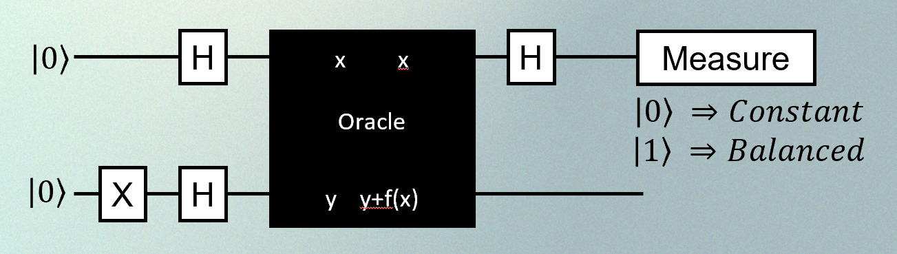
I won’t go through this now (many other places do, and maybe I’ll have a go in Part II, but no promises), but with this circuit just one measurement of the top qubit will tell you whether the black box, labelled here as an “Oracle”, represents a constant or a balanced function. So you can use a combination of superposition and interference to do things you can’t do on a classical computer.
5.3 The canonical algorithms
Since then, a handful of algorithms have been developed that are particularly interesting. The recent book Quantum Computing: An Applied Approach calls them the canon.
These are algorithms for which it has been proved that an ideal quantum computer would offer an algorithm of less complexity than a classical computer.
The big one is the Shor algorithm, which shows how to factor a large number in polynomial time rather than exponential time. And as that is the root of public key encryption schemes there is a lot of excitement.
Another algorithm is the Variational Quantum Eigensolver (VQE). When you see statements like “Quantum computing plays a role in drug discovery and the design of new materials”, this is the technique most aligned with that goal.
A third is the Quantum Approximate Optimization Algorithm (QAOA). When you see claims that “quantum computing will revolutionize logistics and financial portfolio management” this is the technique to think of.
And a fourth is the Grover search algorithm for finding an item in an unstructured database.
But let’s be clear: none of these shows real-world benefit compared to classical computing yet. In particular, despite the progress of quantum computing so far, the biggest number to be factored by a quantum computer a manner that may scale to large numbers seems to be a less-than-impressive 21. And while quantum computing experts say that this does not matter, and that there are technical reasons to focus on other metrics for progress, to me this sounds a bit like they are looking under the street light for their keys.
5.4 Quantum simulation
A side note: you may see some bigger numbers reported for D-Wave systems. There’s no time to talk about that here, but D-Wave is a Canadian company that has taken a different path to quantum computing. It uses quantum simulation, or quantum annealing, which is a separate approach to exploiting quantum phenomena to solve optimization problems. It does not involve gates, and is not a universal model of computation.
I think the idea is that many optimization problems are analogous to finding the ground state of a lattice of qubits (so-called “Ising problems”). The approach is to match the problem of interest to a lattice, build this lattice of qubits in the quantum computing device, cool it down, and see where it settles. Than match that back to the problem of interest to get the solution.
D-Wave have build computers, or simulators, using this approach with superconducting circuits as their qubits. It seems to be true that D-Wave can tackle many problems that other quantum computers cannot, but it remains an open question whether D-Wave machines really show a quantum advantage over classical computers.
6 Quantum computing in 2024
So where are we when it comes to building real quantum computers that can handle problems of interest? There are several metrics of interest: here are three (I’m sure there are others).
Number of qubits. But implicit in the discussion above is that a qubit behaves well: that it is in one well-defined quantum state and stays there. In practice, a distinction is needed between “physical qubits” which may be less-than-perfect, and “logical” or “error-corrected” qubits, which behave properly.
Number of gates. To be able to operate on an array of qubits with a succession of gates is demanding. Not all systems can stay “coherent” for the length of time it takes to apply a number of gates. So it is not at all clear that once you have a large number of qubits, even if they are properly error-corrected, you have a successful quantum computer.
Connectivity. Not all quantum computers allow you to implement the same set of gates, and even if you can, for some a “gate” may be a complex, multi-step operation in practice. And in some architectures / modalities, only qubits “near” each other can be used in a particular gate. And some algorithms assume three-qubit gates, which introduces even more complexity. So you may see reference to “transpiling” algorithms, which means taking a quantum circuit and re-expressing it in terms of the gates that you have at hand on a particular quantum computer.
There is a tension relevant for building quantum computers. You need the whole circuit to be a single state, which means no interference from the environment. Yet at the same time you are poking it and prodding it with these gates, which are very explicit interactions with the environment.
Also: no quantum state is really just two states that you can pick between. There are higher energy states that start to get populated as the temperature increases, and which mess things up.
So error correction is a big part of any quantum computing effort. And typically the answer is the same as any other error correction system: redundancy. So there is a distinction between physical qubits (which are the building blocks we have talked about) and logical qubits, which are collections of physical qubits that you can trust to behave in the way the theory needs. So how many logical qubits to a single physical qubit? Depends on the approach, but the leading work says at least 50.
6.1 Current state of the art
Leading implementations have about a thousand qubits with gate times of 10 ns and what is called “gate fidelity” of three nines. These have all come a long way in the last decade.
Google made big claims four years ago with a 53-noisy qubit processor. They said it could do this task which it would take a classical computer 10,000 years to accomplish. But it’s fundamentally not a very useful task, so no one has really thought much about the best way to do the task on a classical computer. IBM, who is competing with Google of course, came back a short time later and said “we could do that in 2 ½ days”, and another group claimed five minutes. So not convincing yet.
But scale is an important open question. Because we need to get up to at least 10,000 logical qubits to be of any use, and probably into the millions. And despite what Time Magazine says, we are a long way away. And progress is progress, but we can’t assume a Moore’s Law progression yet.
6.2 The big question
So far quantum computing has delivered a set of proofs of concept, together with road maps for scaling up that give an optimistic sense of predictability, when there are still fundamental unknowns to resolve.
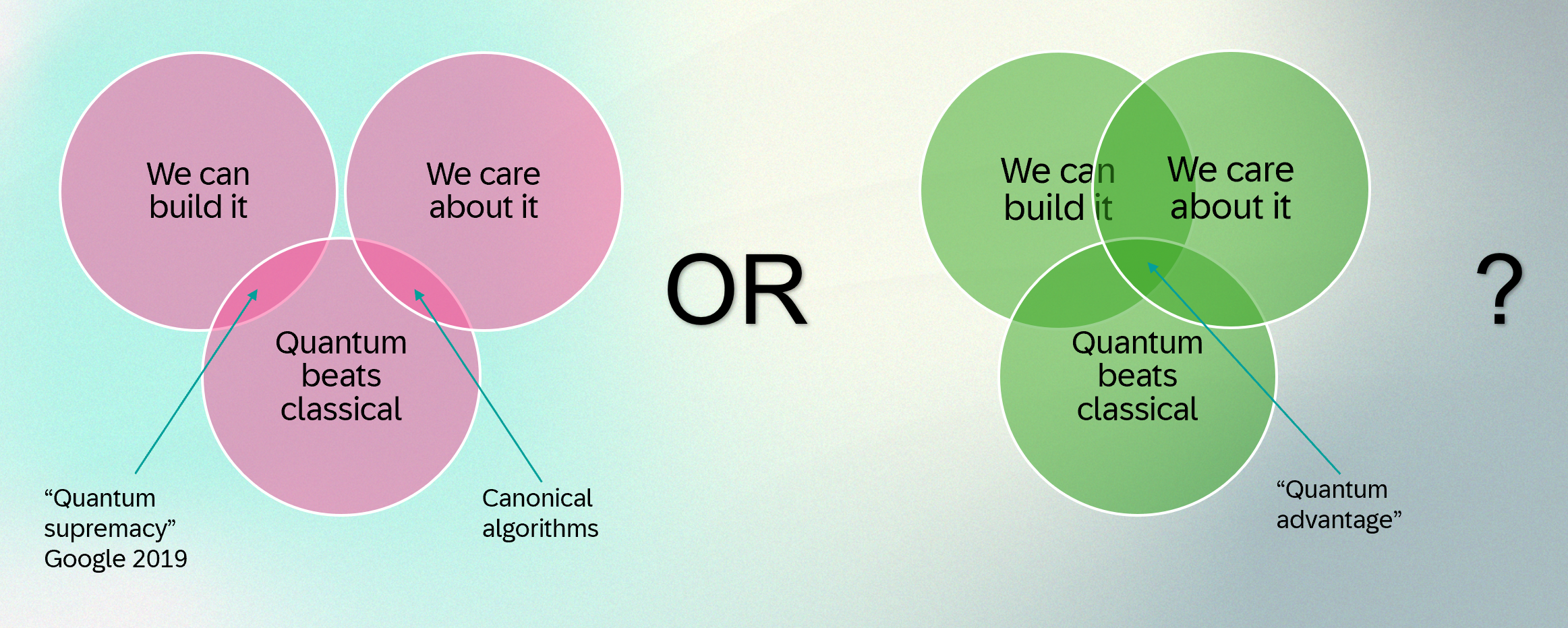
We know there are problems for which there is quantum advantage. We know we can build some of these, like the Google sampling problem, but like the Deutsch algorithm these are mainly artificial. And we know there are problems we care about that have the potential for quantum advantage.
What we don’t know is whether we are on the left or the right side of this diagram. Or, to put it differently, how long we will be on the left side. It’s not a resolved question, and it’s not likely to be resolved soon. But don’t take this from me! Here is a recent quotation from Scott Aaronson, who did a postdoc near me at the University of Waterloo before going on to become one of the leaders in the field of quantum algorithms.
“Billions of dollars [are] being invested in quantum computing… in the hope that a quantum computer would accelerate machine learning, optimization, financial problems, AI problems…. As here, as a quantum algorithms person, honesty compels me to report to you that the situation is much, much iffier.”
Footnotes
There are exceptions: QuEra builds neutral atom quantum computers and says “With an appropriate selection of atomic energy levels for qubit encoding, atoms can even be coherently moved during a calculation”.↩︎
This is not quite true for all modalities: computers built using photonic qubits are not subject to this low-temperature requirement, but they do have other challenges.↩︎
The phrase “basis states” has somewhat different meanings in other areas of quantum mechanics, but usually in quantum computing it refers to the measurement states.↩︎